4.2 Mean Squared Error
We wish to measure the average error between the ultimate losses \(c_u\) and the estimate \(\hat{c}_u\)
\[\begin{align} MSE(\hat{c}_{i,I}) = \mathrm{E}\left[(c_{i,I}-\hat{c}_{i,I})^2 \mid D\right] \end{align}\]
Remark.
Above represents the average error between estimate and actual utlimate given data to date \(D\)
- Standard error: \(s.e. = \sqrt{MSE}\)
Applying the properties of \(\mathrm{Var}(X) = \mathrm{E}[X^2] - \mathrm{E}[X]^2\) we get
\[MSE(\hat{c}_{i,I}) = \mathrm{E}\left[(c_{i,I}-\hat{c}_{i,I})^2 \mid D\right] = \mathrm{Var}\left((c_{i,I}-\hat{c}_{i,I}) \mid D\right) + \left[\mathrm{E}\left[(c_{i,I}-\hat{c}_{i,I}) \mid D\right]\right]^2\]
We can pull out \(\hat{c}_{i,I}\) from the variance and expectation term to get
\[\begin{equation} MSE(\hat{c}_{i,I}) = \underbrace{\mathrm{Var}\left(c_{i,I} \mid D\right)}_{\text{Process Variance}} + \underbrace{\left[\mathrm{E}\left[c_{i,I} \mid D\right] - \hat{c}_{i,I} \right]^2}_{\text{Parameter Variance}} \tag{4.3} \end{equation}\]\(R_i\) is the unpaid for year \(i\):
\[R_i = c_{i,I} - c_{i,k}\]
So the estimate of the unpaid claim is:
\[\hat{R}_i = \hat{c}_{i,I} - c_{i,k}\]
Since the difference between \(\hat{R}_i\) and \(\hat{c}_{i,I}\) is just paid to date (constant) so the MSE are the same
\[MSE(\hat{R}_i) = MSE(\hat{c}_{i,I})\]
4.2.1 Applying the MSE Formula
\[\begin{equation} MSE(\hat{c}_{i,I}) = \left[ s.e.(\hat{c}_{i,I}) \right]^2 = {\hat{c}_{i,I}}^2 \Bigg \{ \sum_{k = I + 1 - i}^{I-1} \frac{{\hat{\alpha}_k}^2}{{\hat{f}_k}^2} \Bigg ( \frac{1}{\hat{c}_{i,k}} + \underbrace{\frac{1}{\sum_{j=1}^{I-k}c_{j,k}}}_{\text{Column x latest}}\Bigg ) \Bigg \} \tag{4.4} \end{equation}\]Remark.
The big \(\sum\) sum over the remaining years till ultimate
- For bit outside the \(\sum\) is same for the row
4.2.1.1 Estimating \(\alpha\)
\(\alpha\) is the proportions for the variance
\[\begin{equation} {\hat{\alpha}_k}^2 = \frac{1}{I - k - 1} \sum_{j=1}^{I-k} c_{j,k} \Big ( \underbrace{\frac{c_{j,k+1}}{c_{j,k}}-\hat{f_k}}_{\text{AY LDFs - Selected}} \Big )^2 \tag{4.5} \end{equation}\]Remark. This one varies by age (columns), for each age:
Calculate the difference2 of the LDFs for each AY and the selected
Then multiply (weight) by each AY’s cumulative loss for given age
- Sum the above and then divide by the number of rows minus 1
\(\alpha^2_{I-1}\) (e.g. \(\alpha^2_9\) for a 10 \(\times\) 10 triangle)
\[\begin{equation} {\hat{\alpha}_{I-1}}^2 = \mathrm{min} \left( {\hat{\alpha}_{I-2}}^2 \times \dfrac{{\hat{\alpha}_{I-2}}^2}{{\hat{\alpha}_{I-3}}^2},{\hat{\alpha}_{I-3}}^2 \right) = \begin{cases} {\hat{\alpha}_{I-3}}^2 & \text{if } {\hat{\alpha}_{I-3}}^2 < {\hat{\alpha}_{I-2}}^2 \\ {\hat{\alpha}_{I-2}}^2 \times \dfrac{{\hat{\alpha}_{I-2}}^2}{{\hat{\alpha}_{I-3}}^2} & \text{else}\\ \end{cases} \tag{4.6} \end{equation}\]Remark. For the last \(\alpha\):
If the 3rd last \(\alpha\) is lower than the 2nd last \(\alpha\), use the 3rd last \(\alpha\)
(If the final \(\alpha\)’s are not trending down, take the lower one)
If the final \(\alpha\)’s are decreasing, then just take the same % of decrease to get the last \(\alpha\)
Also note that if we believe the claims development have stopped at some age \(j\) then we can set \(\alpha^2_j = 0\)
Finally, you can also fit a logarithmic curve to the \(\alpha^2_k\)’s to estimate \(\alpha^2_{I-1}\)4.2.2 MSE Calculation Flow
For a \(10 \times 10\) triangle
Step 1:
Calculate all the \(\hat{f}_k\)
Step 2:
Calculate all the \({\hat{\alpha}_k}^2\)
Calculate a \(\alpha_{i,k}^2\) triangle
- Each cell is \(c_{j,k} \Big ( \underbrace{\frac{c_{j,k+1}}{c_{j,k}}-\hat{f_k}}_{\text{AY LDFs - Selected}} \Big )^2\)
\({\hat{\alpha}_k}^2\) is the sum of column \(k\) over the number of cells - 1
See special case for the last \(\alpha_k^2\)
Step 3:
Calculate the projected triangle using the \(\hat{f}_k\)
Step 4:
Calculate a \(MSE(\hat{c}_{i,k+1})\) triangle
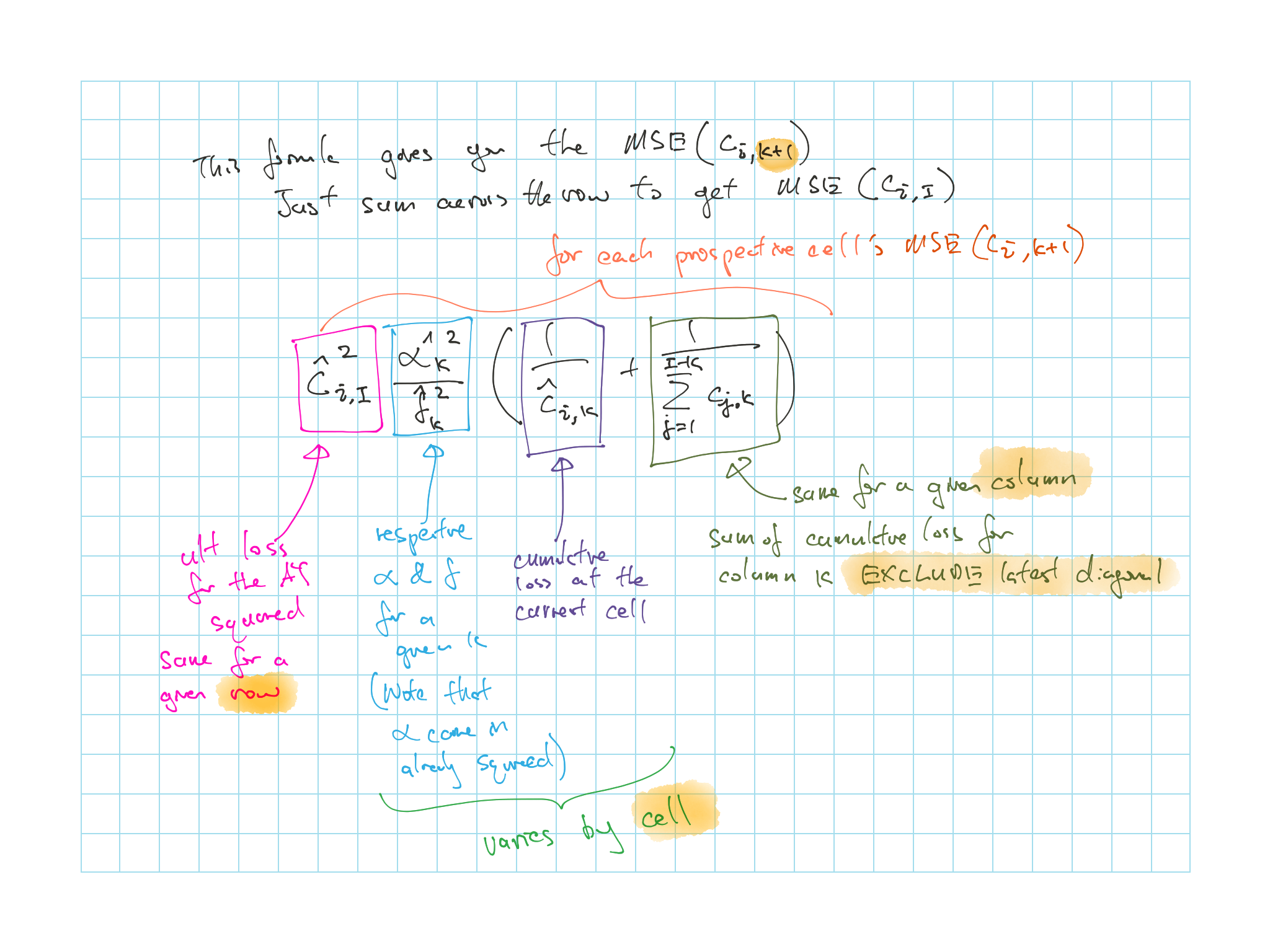
Figure 4.1: Breakdown of MSE formula for each cell
Step 5:
Get the \(MSE\) for the AY by summing up a given row of \(MSE(\hat{c}_{i,I})\)
Step 6:
Get the total \(MSE\) for the total reserve (all AYs) you have to consider the dependencey between AYs since we use the same LDFs