10.5 Stochastic Column Parameters for Bayesian BF

BF above uses stochastic row parameters \(x_i\) and deterministic column parameters (Vol. Wtd. average LDFs)

We can use stochastic process for both by first estimating the column parameters then the row parameters

• Define improper prior distribution for the column parameters first before applying prior distributions for the row parameters and estimating them

• This approach allows us to take into account the fact that the column parameters have been estimated when calculating the prediction errors, predictive distribution etc

• We don’t have to include any information about the column parameters so we use improper gamma distribution (wide variance) for the column parameters

Result posterior distribution:

\[\begin{equation} \begin{array}{c} c_{ij} \mid c_{1,j}, c_{2,j},..., c_{i-1,j}, x, \varphi \sim ODNB \\ \mathrm{E}[c_{ij}] = (\gamma_i - 1) \sum \limits_{m=1}^{i-1} c_{m,j} \\ \end{array} \tag{10.13} \end{equation}\]

• Note that it is similar to (10.6) but recursive down the column (over \(i\))

  • \(\sum \downarrow\)

• \(\gamma_i\) is the new row parameters

  • This tells you the level of losses in the row relative to the rows above

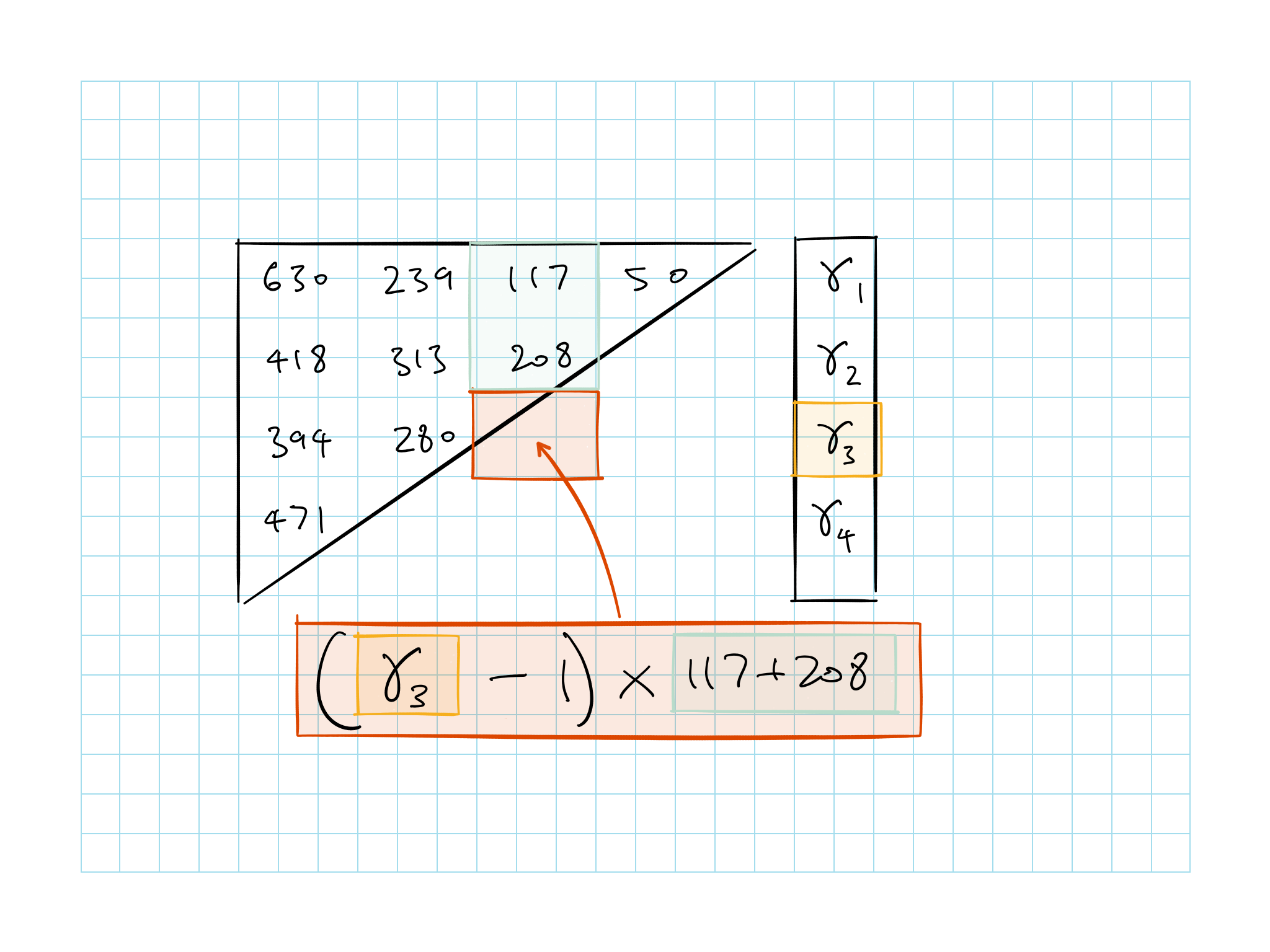
Figure 10.1: Stochastic Column Parameters

We now have a stochastic version of the BF method

• BF inserts values for the expected ultimate claims in each row, \(x_i\), in the form of the values \(M_i\)

• In Bayesian context, prior distributions will be defined for the parameters \(x_i\) as discussed above

• However, the model has been reparameterized with a new set of parameters \(\gamma_i\)

• Therefore it is necessary to define the relationship between the new parameters \(\gamma_i\) and the original \(x_i\)

• Section below shows how to find \(\gamma_i\) from the values of \(x_i\) given in the prior distributions

Stochastic BF summary:

• Column parameters (LDFs) are dealt with first using improper prior

  Their estimates will be those implied by the Chainladder

• Prior information can be defined in terms of distributions for the parameters \(x_i\), which can then be converted into values for the parameters \(\gamma_i\)

10.5.1 Calculate Gamma

Know how to calculate this pictorially (equation is complicated…)

First, use Chainladder to get ultimate loss and % unpaid by AY

\[\gamma_1 = 1.000\]

First calculate LDFs, then the % unpaid and a-priori for each AY

• \(U_i\) = a-priori ultimate based on LDF for AY \(i\)

• \(q_i\) = % unpaid for AY \(i\)

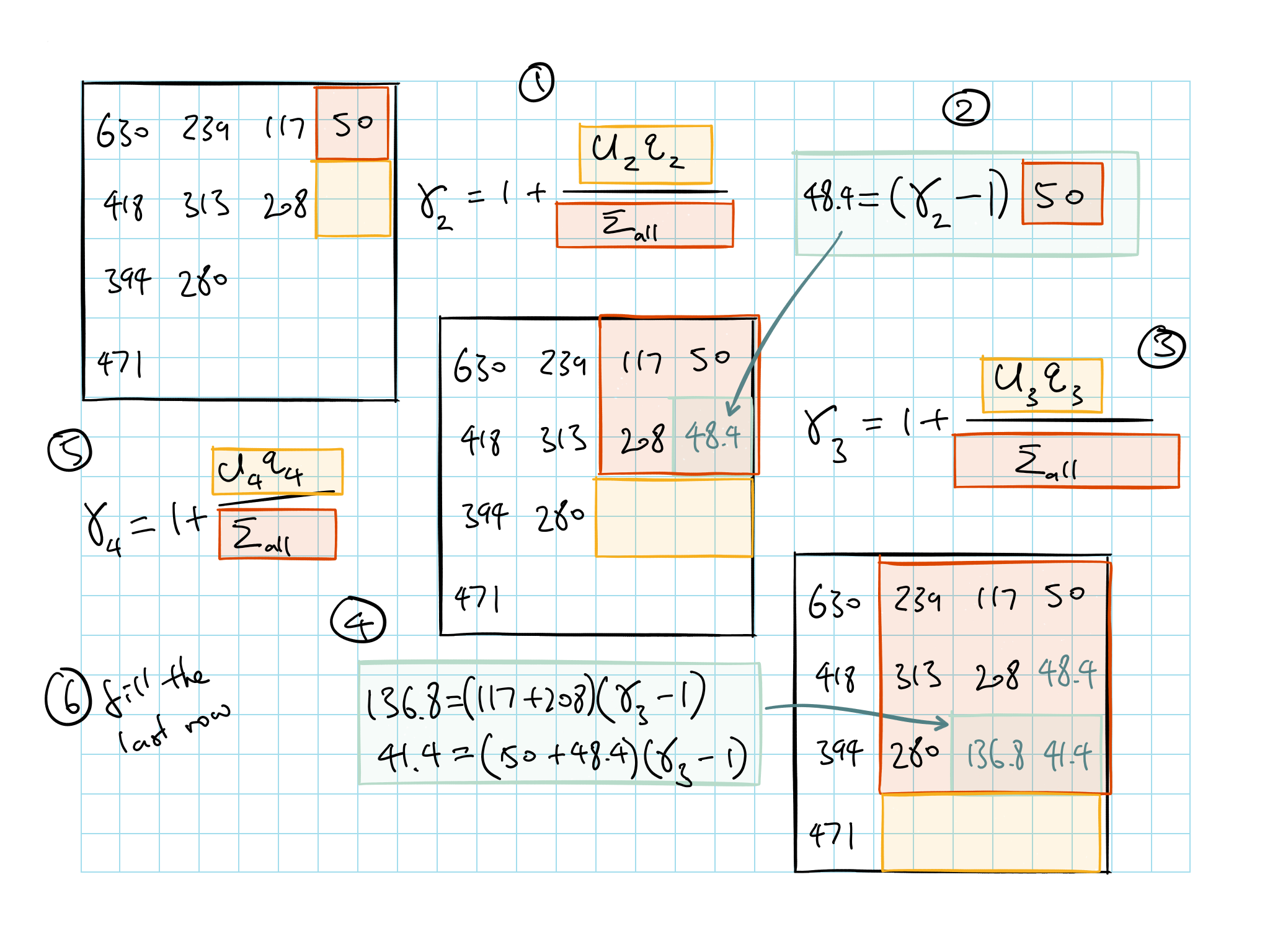
Figure 10.2: Calculating gamma

Note that in step 4 above if you don’t need the individual cells you can just take the \(U_3 q_3\)