CAS Exam 7 Study Notes

5.4 Implication 2: Superiority of Alternative Emergence Patterns

If an alternative emergence pattern provides a better explanation of the triangle, maybe it should be used

Table 5.3: Alternative emergence pattern on a \(m \times m\) triangle
Emergence Patterns	# of Parameters \(p\)	Comments
\(\mathrm{E}[q(w,d+1) \mid \text{Data to }w+d] = f(d) c(w,d)\)	\(m - 1\)	e.g. Chainladder
\(\mathrm{E}[q(w,d+1) \mid \text{Data to }w+d] = f(d) c(w,d) + g(d)\)	\(2m - 2\)	e.g. Least Squares
\(\mathrm{E}[q(w,d) \mid \text{Data to }w+d] = f(d)h(w)\)	\(2m-2\)	e.g. BF
\(\mathrm{E}[q(w,d) \mid \text{Data to }w+d] = f(d)h\)	\(m-1\)	e.g. Cape Cod

Remark. \(f(d) c(w,d) + g(d)\)

Remark. \(f(d)h(w)\)

Here \(f(d)\) is related to the % of losses emerged in period \(d\)

Incremental % emergence, NOT LDF - 1
\(h(w)\) can be think of as an estimate of ultimate losses for AY \(w\)

Like an a-priori
The -2 for the BF is due to \(f(0)\) and constant (degrees of freedom?)
If BF is better \(\Rightarrow\) Loss emergence is more accurately represented as fluctuating around a proportion of expected ultimate losses (rather than proportion of reported losses)
Cape Cod works when the loss ratio is stable (stable book of business)
- Use \(h(w) = h \times Premium(w)\), so we only need stable ELR
- Cape Cod works out to an additive model \(q(w,d) = h \times f(d)\)
Can further reduce parameters by combining some row and column parameters
- Might be intuitively appealing to sum up the recent and tail years of the \(h(w)\) since there’s little empirical data to support different estimates
We’ll be mostly focusing on this form

Consider \(\mathrm{E}[q(w,d) \mid \text{Data to }w+d] = f(d)h(w)\) from Table 5.3

We need to minimize the sum of squared residuals to get the optimal \(f(d)\) and \(h(w)\):

\[\sum_{w,d} \varepsilon^2(w,d) = \sum_{w,d} [q(w,d) - \underbrace{f(d)h(w)}_{\mathrm{E}[q(w,d)]}]^2\]

Remark.

Since this is a non-linear model, we need an iterative method to minimize to SSE
We can use weighted least squares if the variances of the residuals are not constant over the triangle

We need to minimize the variance of each residual \(\varepsilon(w,d)\)

\[\mathrm{Var}(\varepsilon(w,d)) \propto f(d)^p h(w)^q\]

Remark.

\(p\) & \(q\) typically \(\in [0,1,2]\)
And regression weights (applied to each \(f(d)\) or \(h(w)\)) will be \(\dfrac{1}{f(d)^p h(w)^q}\) (inversely proportional to variance, similar to Mack 1994)

Since \(\mathrm{E}[q(w,d)] = f(d)h(w)\)

\(f(d) = \dfrac{\mathrm{E}[q(w,d)]}{h(w)}\), and
\(h(w) = \dfrac{\mathrm{E}[q(w,d)]}{f(d)}\)
So the actual \(\dfrac{q(w,d)}{h(w)}\) is an estimate of \(f(d)\) and vice versa
And we can estimate \(f(d)\) based on a weighted average of each observation

Different variance assumption for \(\varepsilon\) \(\Rightarrow\) different parameters (weight) similar to the Chainladder method in table 5.2

Table 5.4: Variance and parameters for various form of \(\mathrm{E}[q(w,d) \mid \text{Data to }w+d] = f(d)h(w)\)
Method	\(\mathrm{Var}(\varepsilon(w,d)) \propto f(d)^p h(w)^q\)	\(\mathbf{f(d)}\): Col Parameters	\(\mathbf{h(w)}\): Row Parameters
BF¹	\(p=q=0\)	\(f(d) = \dfrac{\sum_w h^2 \frac{q}{h}}{\sum_w h^2}\)	\(h(w) = \dfrac{\sum_d f^2 \frac{q}{f}}{\sum_d f^2}\)
Cape Cod²	\(p=q=0\)	\(f(d) = \dfrac{\sum_w h^2 \frac{q}{h}}{\sum_w h^2}\)	\(h = \dfrac{\sum_\Delta f^2 \frac{q}{f}}{\sum_\Delta f^2}\)
BF (Var \(\propto\) \(fh\))³	\(p=q=1\)	\(f^2(d) = \dfrac{\sum_w h \left( \frac{q}{h} \right) ^2}{\sum_w h}\)	\(h^2(w) = \dfrac{\sum_d f \left( \frac{q}{f} \right)^2}{\sum_d f}\)

BF: assumes each \(q(w,d)\) have constant variance (least square, standard regression)

For \(h(w)\) weight is \(f(d)^2\) and cells with higher expectes loss get higher weight

For \(f(d)\) weight is expected ultimate losses squared, years with higher expected losses get higher weight
Cape Cod: also assumes constant variance
Variance of the cell is proportional to the expected loss of the cell

Recall from Mack 1994, we need to look at the residual graphs to determine which variance assumption is appropriate

Need to seed one of them and iterate until convergence

e.g. for constant variance BF: \(f(d)\) \(\sum \downarrow\); \(h(w)\) \(\sum \rightarrow\)
Use the above to estimate the parameters and then calculate the unpaid
When combining parameters, don’t count the \(f(0)\) and always subtract 1

Step 1) Start iteration with the \(f(d)\) from Chainladder

Step 2) Find \(h(w)\)’s that minimize the \(SSE\)

Step 3) Find \(f(d)\)’s that minimize the \(SSE\) based on the \(h(w)\) from step 2

Step 4) Repeat step 2 & 3 till convergence

Step 5) Use the \(f(d)\) and \(h(w)\) calculated to get the estiamted triangle to calculate \(SSE\) or do projection

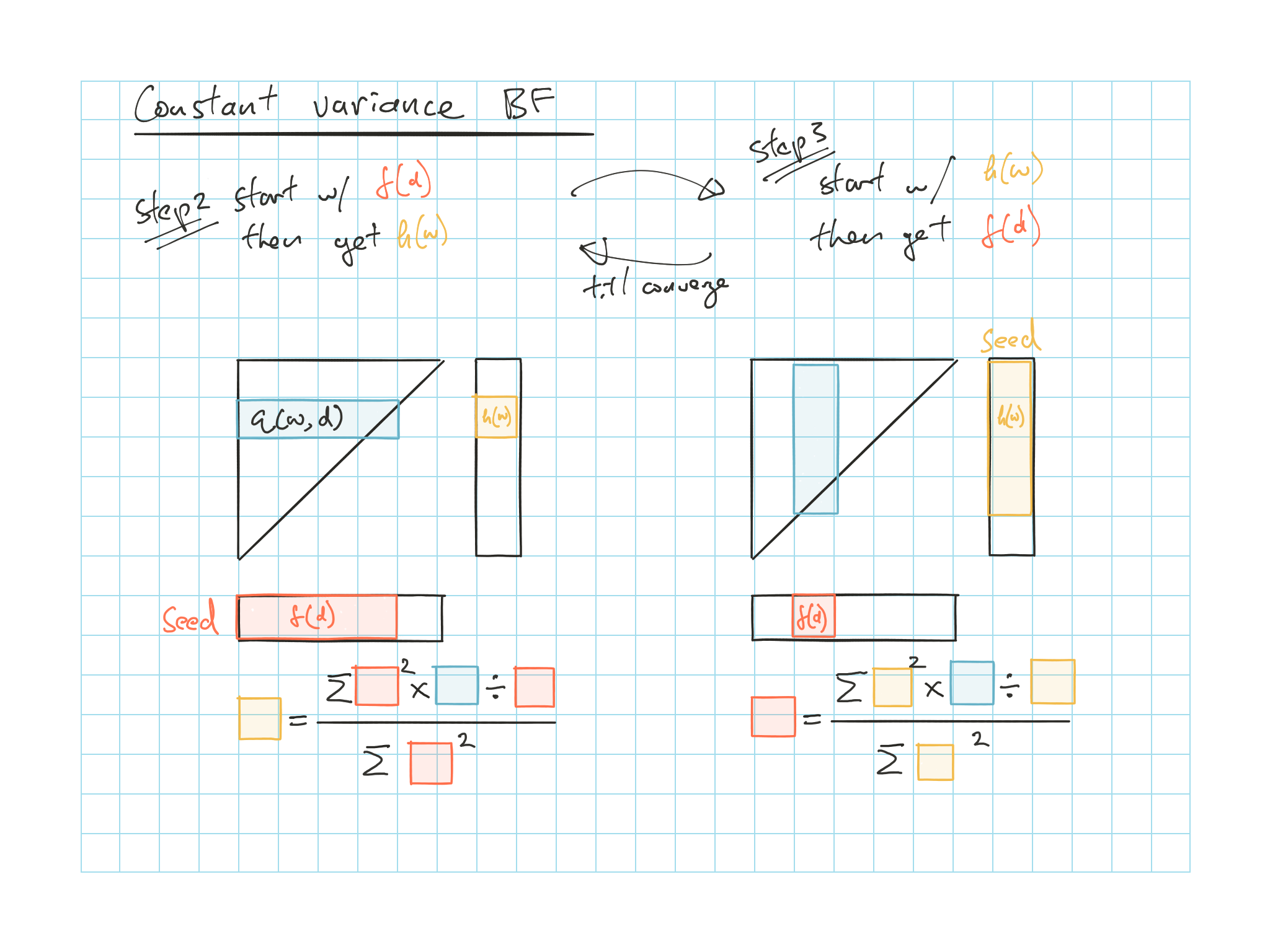
Figure 5.1: BF with constant variance

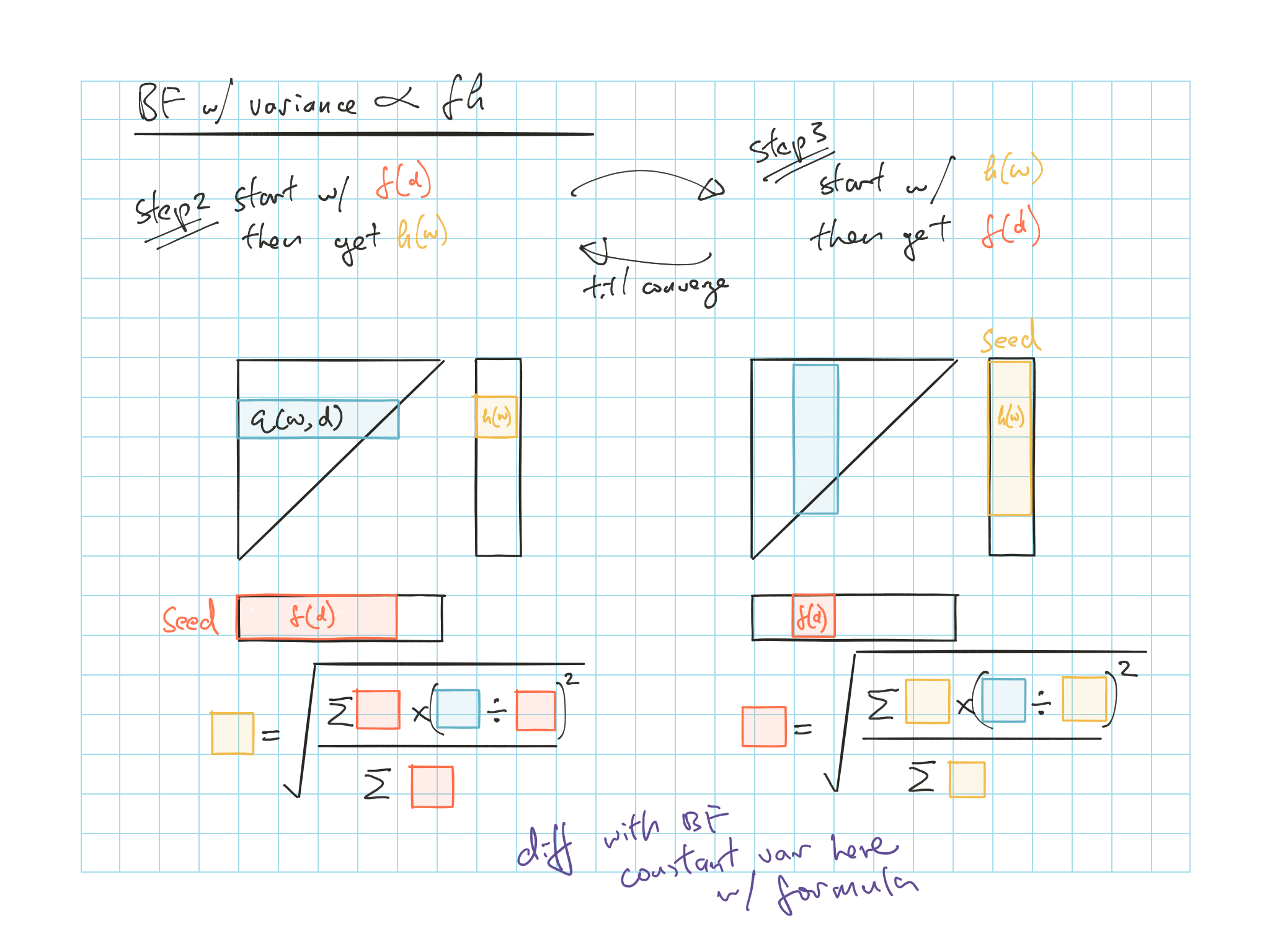
Figure 5.2: BF with variance proportional to \(fh\)

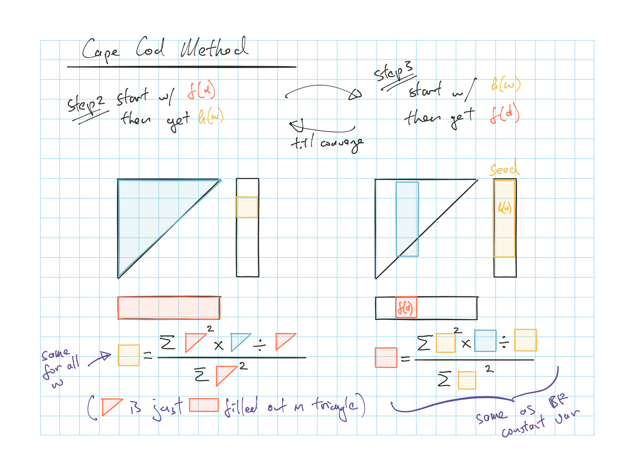
Figure 5.3: Cape Cod

For n

For reserving: number of cell in the triangle minus the first column \(\dfrac{m(m-1)}{2}\)

(Since we don’t need to forecast the first column to calculate the unpaid)
For pricing: number of cell in the triangle

For p (Just a walk through of how we get the \(p\) in Table 5.3)

BF: Start with \(2m\) parameters all the \(f(d)\)’s and \(h(w)\)’s
1. We don’t need \(f(0)\) for reserves again since we don’t need to forcast the first column
2. Less one more due to degree of freedom
  
  (Since you can fix any one of the parameters and still get the same results)
3. So we have \(p = 2m-2\)
Similarly for Cape Cod but we only start with \(m + 1\) so we ended up with \(m-1\) (i.e. taking out the \(f(d)\) and the degree of freedom)
Grouped BF is similar as well if you don’t group the \(f(0)\)
- Note: If you group the \(f(0)\) you can’t subtract one for that as you’ll be using the parameter
Chainladder you have \(m\) for all the \(f(d)\)’s to start with and less the \(f(0)\)