11.3 Testing Procedure
We are testing the process of each method and not the results of any one distribution generated from the method
Since there’s only 1 actual outcome for each triangle we test
Focus on the process (the different methods) that gives us the distribution
Compare the predicted percentiles (from the methods) against the expected percentile
Typically we can compare distributions by comparing the density function, but we can not in this case because 1) We have a small data sets (50 points) 2) Each data point comes from a different distribution
Testing Procedure
Given \(N\) triangles and their actual outcome in 10 years
Generate \(N\) sets of distribution (from the \(N\) triangles using one of the methods) and determine the predicted percentile \(p_i\) based on the predicted distribution
- i.e. see where the actual outcome lands on our predicted distribution
The distribution of the \(N\) predicted percentiles \(p_i\) should follow a uniform distribution if the model is accurate, so we rank them to form \(\{p_i\}\)
\[\{p_i\} = \{p_1,...,p_n\}\]
- The expected percentiles \(\{e_i\}\) should run from \(\frac{1}{n+1}\) to \(\frac{n}{n+1}\)
\[\{e_i\} = \left\{ \dfrac{1}{n+1}, \dfrac{2}{n+1},...,\dfrac{n}{n+1} \right\}\]
11.3.1 Kolmogorov-Smirnov Test
For the KS test we’ll compare \(\{ p_i \}\) with \(\{ f_i \}\)
\[\begin{equation} \{f_i\} = \left\{ \dfrac{1}{n}, \dfrac{2}{n},...,\dfrac{n}{n} \right\} \tag{11.1} \end{equation}\]\(H_0\): Distribution of \(p_i\) is uniform
Test statistics for maximum difference between the predicted and expected percentiles
\[\begin{equation} D = \max \limits_i \mid p_i - e_i \mid \tag{11.2} \end{equation}\]Reject \(H_0\) @5% confidence level if:
\[\begin{equation} D > \dfrac{136}{\sqrt{n}}\% \tag{11.3} \end{equation}\]- i.e. For \(n = 50\) \(\Rightarrow\) 19.2%; \(n=200\) \(\Rightarrow\) 9.6%
Example
| \(f_i\) | \(p_i\) | \(abs\{ p_i - f_i \}\) |
|---|---|---|
| (1) | (2) | (3) |
Col (1): \(\{f_i\} = \left\{ \dfrac{1}{n},...,\dfrac{n}{n}\right\}\)
Col (2): \(\{p_i\}\) = \(p_i\) from each realization of the triangles sorted in ascending order
Col(3) = Absolute difference between the first two columns
\(D\) is the maximum value from column (3)
Compare \(D\) with \(\dfrac{136}{\sqrt{N}}\)
If \(D\) is less than the critical value we do not reject the \(H_0\) that \(\{ p_i \}\) is uniform
Remark. Technically based on Klugman you test against both:
\[\{f^+_i\} = \left\{ \dfrac{1}{n}, \dfrac{2}{n},...,\dfrac{n}{n} \right\}\]
and
\[\{f^-_i\} = \left\{ \dfrac{0}{n}, \dfrac{2}{1},...,\dfrac{n-1}{n} \right\}\]Alternatively, we can use Anderson-Darling test that focuses on the tail
- But it failed all the models therefore we do not use it as it does not help in model comparison
11.3.2 p-p Plot
We plot the \(p-p\) plot with \(e_i\) vs \(p_i\) to diagnosis
Dark blueline is what is expected from uniform distribution
Light blueline is the critical value for a given \(n\) from the KS test above
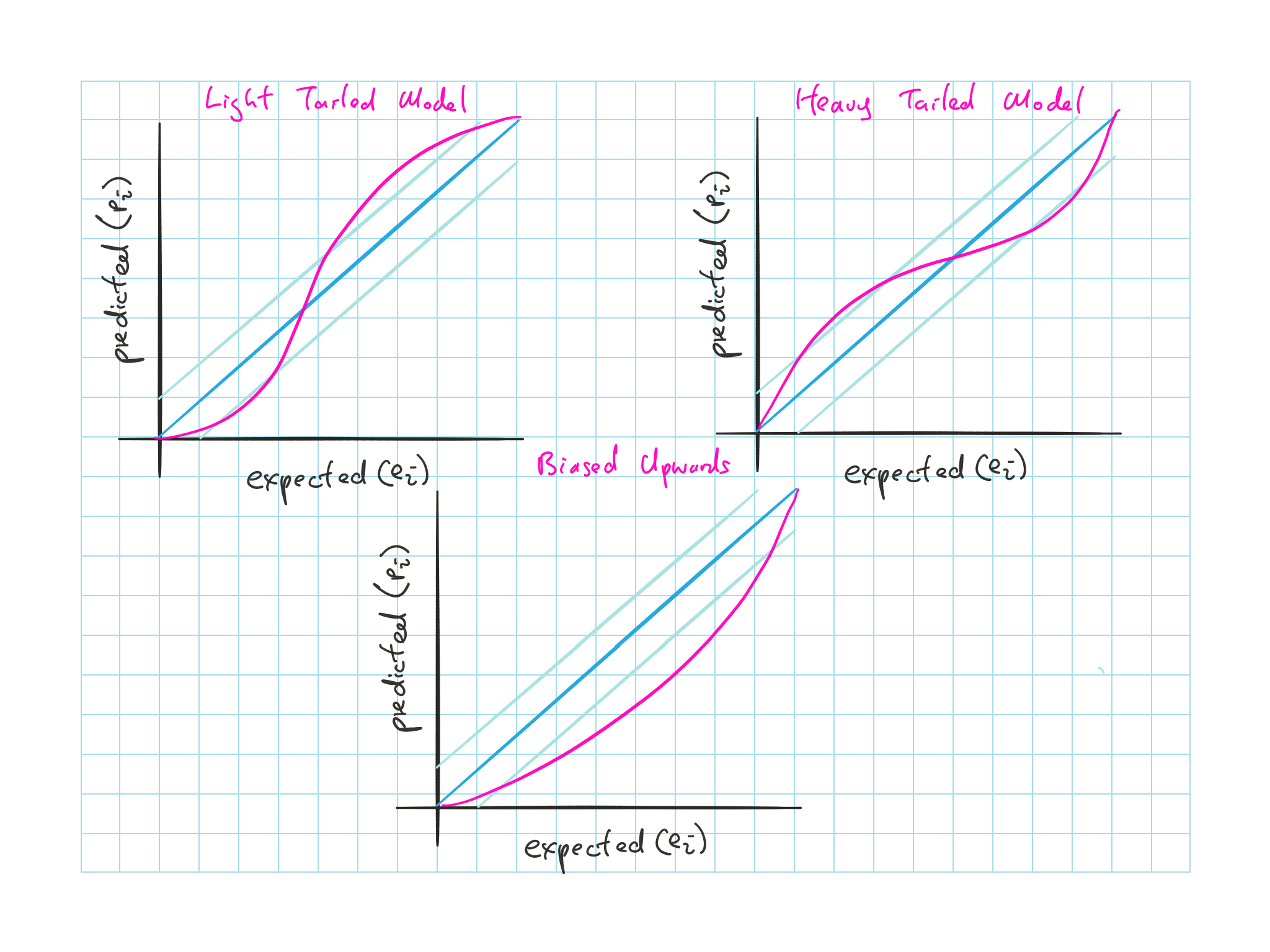
Figure 11.1: p-p plot
Model is too light tailed: Shallow slope near corner and steep in the middle
Model is too heavy tailed: Steep slope near corner and shallow in the middle
Model is biased upwards: Bow down
- Biased upwards: predicted mean > true mean while the s.d. is correct
If we look at lognormal data fitted to normal, we’ll see a mix of light and heavy tailed model
- i.e. The right tail will be too light so we’ll see a shallow slope in the right and the left tail will be too light so we’ll see a steep slope at the left
11.3.3 Percentile Histogram
We plot a (flipped) histogram
y-axis being the predicted percentile
x-axis is the frequency
Bins with width 0.1 (so 10 bins)
Vertical blue line represent the expected frequency based on uniform \(\{e_i\}\)
- Expected frequency = \(\dfrac{\text{# of points}}{\text{# of bins}}\)= \(\dfrac{n}{10}\)
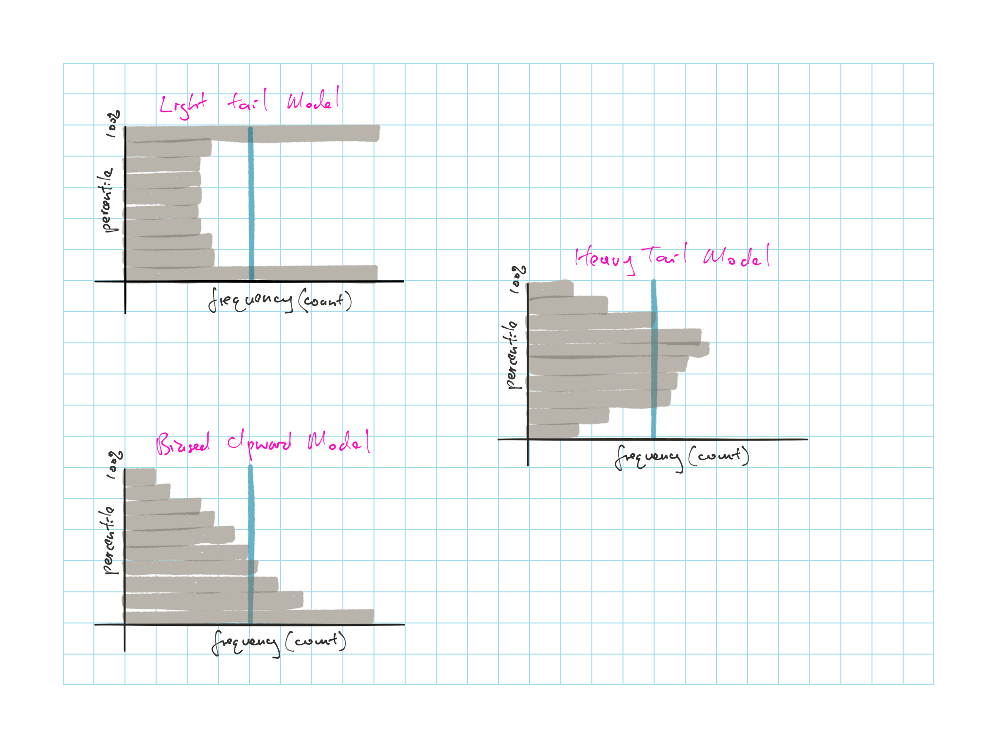
Figure 11.2: Percentile Histogram