13.3 Reinsurance Reserving Procedure
Partition \(\Rightarrow\) Development Patterns \(\Rightarrow\) Estimate \(\Rightarrow\) Monitor and AvE
Partition into homogeneous exposure groups that are consistent over time with respect to mix of business
Analyze historical development; Ideally, consider case and emergence of IBNR claims separately
Estimate future development; Ideally, estimate IBNER and pure IBNR separately
Monitor and testing predictions (AvE)
13.3.1 Step (1): Portfolio Partition
Data needs to be split into reasonably homogenous exposure groups that are relatively consistent over time with respect to mix of business (exposures)
- Group policies with similar report lags and development profile
Variables to consider when partitioning data in approximately priority order:
LoB
Contract type (fac, treaty, finite)
Types of Cover (QS, SS, XS per risk/occ, agg XS, CAT, LPT)
Primary LoB (for cas)
Attachment Point (for cas)
Contract terms (flat-rated, retro rated, sunset clause, LAE share, CM, Occ)
Type of cedant (Small, large, E&S)
Intermediary (brokers)
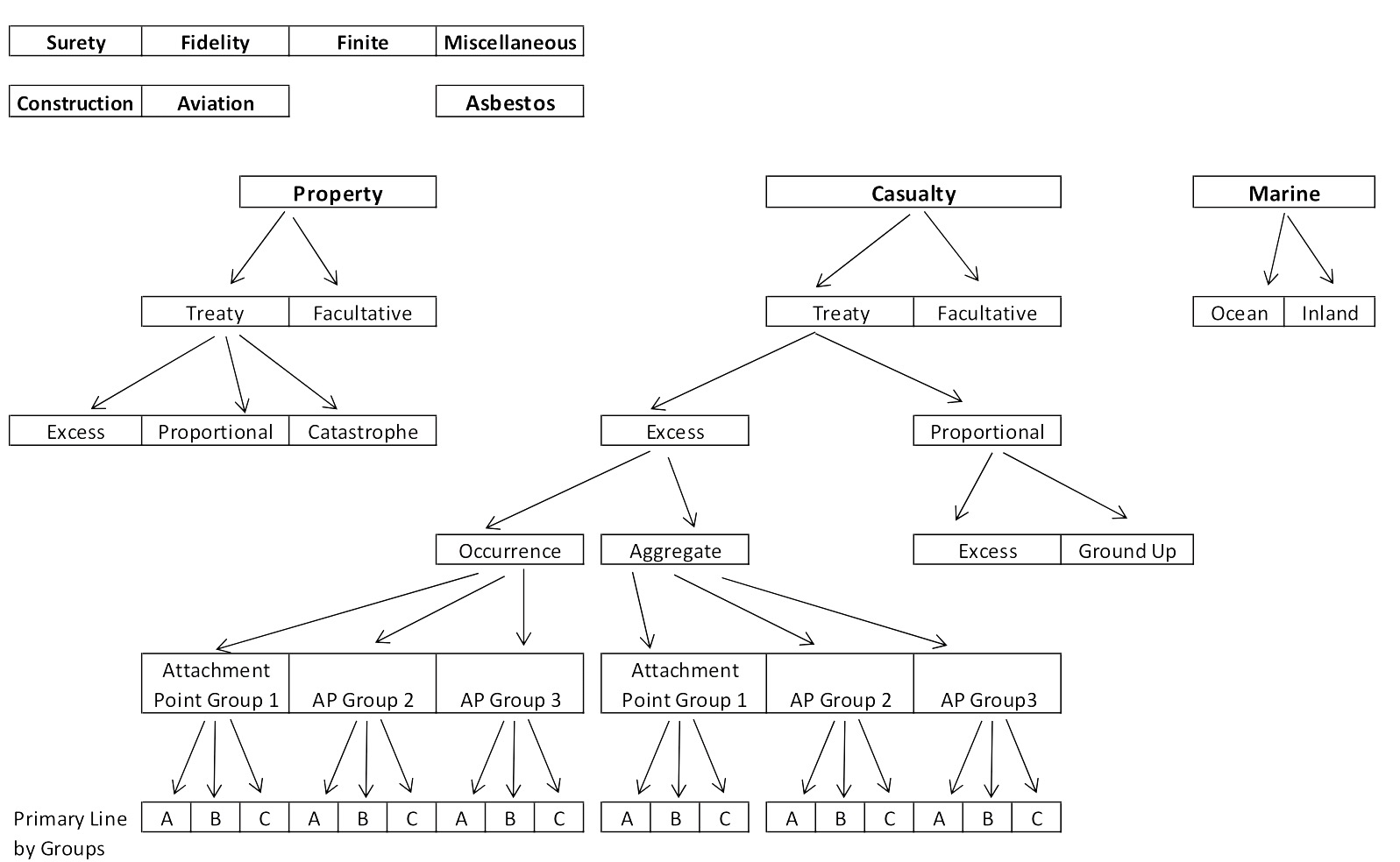
Figure 13.1: Portfolio Partition
Example:
Start with the LoB or some other major categories
Further breakdown into fac or treaty
All significant XS exposure should be further broken down by type of retention (e.g. per-occ XS vs agg XS)
Treaty casualty XS should be further broken down by attachment point range and primary LoB (e.g. AL, GL, PL, WC, etc)
Treaty casualty proportional should be broken down by first dollar primary layers (group-up) vs higher excess layer (excess)
- Do we also breakdown by primary line?
Facultative casualty: breakdown by automatic primary programs (pro rata share of group-up exposure) vs automatic nonprimary programs (excess)
Certificate exposure should ideally be split by attachment point range
- Or at least buffer vs umbrella layer and then further by primary line
For property and other exposure: split by pricing categories
Need to balance homogeneity with credibility of data
Review loss statistics and reporting pattern to see if data is still credible
Leverage u/w-er, claim handlers and data processors to determine which variables are the most important
13.3.2 Step (2) & (3): Analyze Historical Data and Projection
Backward looking of historical data (Step 2):
Analyze the historical development patterns. If possible, consider individual case reserve development and the emergence of IBNR claims separately
- Use long periods where practical and curve fit where practical
Forward looking and projection (Step 3):
Estimate the future development. If possible, estimate the bulk reserve for IBNER and pure IBNR separately
13.3.2.1 Claim Report and Payment Lags
We want to find stable expected development pattern for homogeneous categories
Definition 13.1 \(y = Rlag(t) = p_k\) (\(p_k\) is the Clark notation)
Report lag \(= \dfrac{1}{ATU \text{at time }t} =\) % Reported to DateRemark. Benefits of the above definition:
We can fit a parametric curve (see Clark) to smooth curves to compute the tail
e.g. Gamma with \(\mu\) = 2.5 years and \(\sigma\) = 1.5 years (Figure 13.2)
\(Rlag(t)\) can be interpret as probability that any particular claims dollar will be reported to the reinsure by time \(t\)
- We can compute statistics such as the expected value to compare one claim report pattern with another
##
## Attaching package: 'dplyr'
## The following objects are masked from 'package:stats':
##
## filter, lag## The following objects are masked from 'package:base':
##
## intersect, setdiff, setequal, union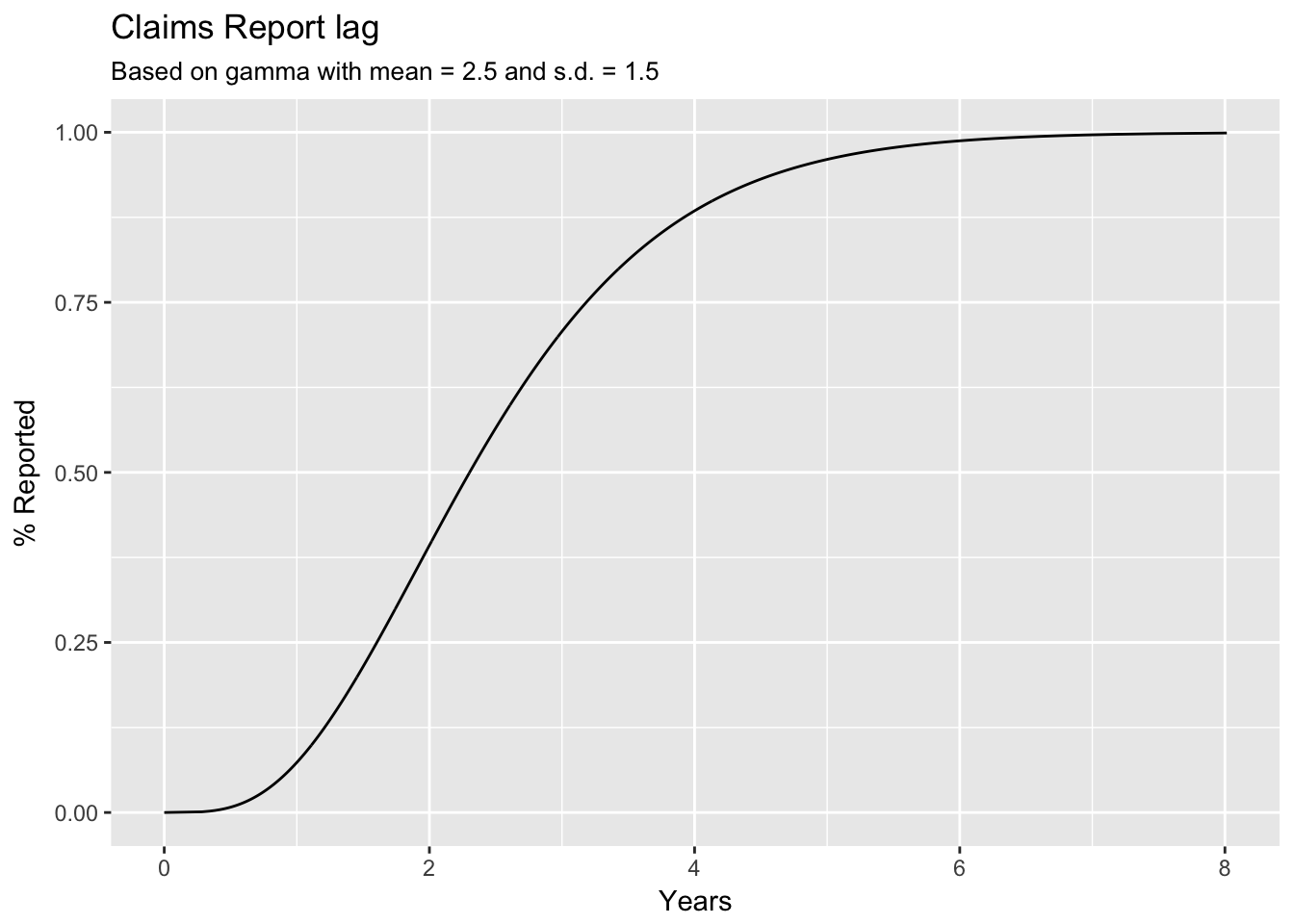
Figure 13.2: Claims report lag based on Gamma distribution
13.3.2.2 Short Tailed Lines
Loss reporting and settlement is quick
\(\therefore\) Use method that provide reasonable accuracy for the least effort and cost
| Category I1 | Category II | Category III |
|---|---|---|
| Property | Treaty | Proportional |
| Property | Treaty | Cat |
| Property | Treaty | Excess2 |
| Property | Facultative3 | |
| Fidelity | Proportional |
For property, beware of recent cat events
Exclude high layers for XS property
Exclude construction
- International exposure can have significant reporting delay as well
Estimation Methods
Set IBNR = % of the last 12 months’ EP
Reasonable for non-major-cat “filtered” claims
Claims for major cat may not be fully reported and finalized for years even on proportional covers
Book LR for new lines
Allocate claims to AY for reserving (based on historical information)
U/w year (or treat year) will have extra lag
Treaty effective 1/1/16 will cover policies inception from 1/1/16 to 12/31/16 and therefore can cover accidents that happens in 12/31/17 \(\Rightarrow\) 2 years after the inception of the treaty
13.3.2.3 Medium Tailed Lines
Definition 13.2 Medium-taild exposure
Average dollar lag of 1-2 years
Almost completely settled within 5 years
- Over half the ultimate losses are reported within 2 years
| Category I | Category II | Category III | Category IV |
|---|---|---|---|
| Property | Treaty | Excess | High layers1 |
| Construction2 | |||
| Surety | |||
| Fidelity | Excess | ||
| Ocean Marine | |||
| Inland Marine | |||
| Property | International | ||
| Non-casualty | Excess | Aggregate3 |
Ideally separate from working layers
- Ultimate value may not be known immediately and will take longer to penetrate higher per-risk XS attachment point
Ideally separate from other property exposures
- Discovery period can extend years beyond the contract period
Lags are longer then the underlying exposure
For surety should estimate gross and recovery separately as the recovery has a longer tail
- Consider the ratio of salvage to gross loss for mature years
Estimation Methods
- Chainladder works fine for paid and incurred with or without ACR
13.3.2.4 Long Tailed Lines
Definition 13.3 Long-taild exposure
Exposures which the average aggregate claims dollar report lag is over 2 years
- Claims are not settled for many years
| Category I | Category II | Category III | Category IV |
|---|---|---|---|
| Casualty | Treaty | Excess1 | |
| Casualty | Treaty | Proportional2 | |
| Casualty | Facultative | ||
| Casualty | Excess | Aggregate3 | |
| APH4 |
Longest lags except for APH
Some of this exposure maybe medium-tailed
Lag are longer than for the underlying exposure
Asbestos, pollution, and other health hazard and mass tort claims
Longest of the long tail
Should be remove from data and analyzed separately
Use methods specifically for APH
Exclude claims from commuted contracts as they distort development patterns
- Need to separate the above into finer, more homogeneous categories (e.g. separate claims-made and occurrence coverage)
13.3.2.4.1 Long Tailed Lines: Estimation Methods
Chainladder (CL):
Don’t use, too much leverage
Bornhuetter-Ferguson (BF):
Better than CL, correlate future development with an exposure measure (reinsurance premium): Premium \(\times\) ELR
Caveat 1): Very dependent on selected LR
LR for a given AY is strongly correlated with the underwriting cycle as well as the reported loss to date
\(\therefore\) need to consider the u/w cycle in ELR pick
(May use LR from pricing work)
Caveat 2): Estimate for each AY does not reflect the reported to date
(unless the selected LR is chosen with that in mind)
Stanard Buhlmann (SB or Cape Cod in Europe):
\[ELR = \dfrac{\sum C_k}{\sum E_k p_k}\]
\(C_k\): reported to date
\(E_k\): Adj Prem
\(p_k\): expected % reported to date
\(k\) is the exposure year
Must on-level the historical premium and adjust to be pure premium (\(E_k\))
Remove commissions and brokerage and internal expenses (but might not worth the effort)
Remove any suspected rate level differences (so each year have the same ELR)
We need to do this because we are using a constant expected LR for all AYs
Unclear how to adjust ELR to a prior estimate for each year (from 2000 #68)
SB IBNR:
\[\begin{align} IBNR_k &= E_k(1-p_k) \times ELR \\ &= (E_k - p_k E_k) \times ELR \\ \end{align}\]
For all years \(IBNR\) we have
\[\begin{align} IBNR &= \sum_k (E_k - p_k E_k) \times ELR \\ &= \left( \sum_k E_k - \sum_k p_k E_k \right) \times ELR \\ &= (\text{Total Adj Prem} - \text{Total Used Up Prem}) \times ELR \\ &= \text{Premium Not Used} \times ELR \\ \end{align}\]
Remark.
This estimate of the ELR use actual incurred loss
Method is sensitive to the accurary of the on-level EP
- Total used up premium is something we’ll already have from calculating the \(ELR\)
Credibility IBNR Estimates
Weight the CL method with SB or BF
Reserve (or IBNR) for year \(k\):
\[\hat{R}_k = Z_k \times R^{CL}_k + (1-Z_k)\times R^{SB}_k\]
\(Z_k = p_k \times CF\); Credibility Factor \(CF \in [0,1]\)
\(CF = 0\) \(\Rightarrow\) BF
\(CF = 1\) \(\Rightarrow\) Benktander (GB)
Can also weight together the IBNR estimate from paid loss method
- Case reserve are based on judgement of many people and can vary over time (lack consistency) \(\Rightarrow\) Given long enough paid history, paid estimate might be more stable and credible
Or weight with BF based on different a-priori (e.g. based on pricing ELR)
Alternative Methods
Fit losses reported to date to a curve (Clark)
- Practical problem:
Negative incrementals (get around by grouping over different periods)
Model claim counts and use stochastic model (Bootstrap) for the whole claims development process
Caveat: difficult to explain to management
Advantage: Can contemplate intuitively satisfying models for various lag distributions
Time from loss to first report and lag from report to settlement
Connect the lags with appropriate models for the dollar reserving and payments on individual claims up through settlement
13.3.3 Step (4): Monitoring and Testing Predictions
Compare AvE over quarters and do this for several quarters to see if any trends become apparent
Forecast IBNR runoff over the quarters
Provides early warning if claims are emerging higher than expected
Definition 13.4 Expected reported claims
\(\dfrac{\text{Expected % Reported in Period}}{\text{Expected % Unreported}} \times IBNR\)Caveat:
Can be difficult to tell if the AvE difference is large or small
\(\therefore\) Look for deviations over time and look for trends
Deviation could be IBNR is too small, claims are paying faster than expected, or just random fluctuation